The derivative of a function can be thought of as the rate of change of the function. If the function represents the position of a particle then the derivative would be the velocity of the particle.
The usual approach is to define the derivative as a limit. This requires defining limits, and proving various properties, and then applying that to the derivative and proving further theorems about the derivative.
As an alternative, we will start with approximating a function by a straight line. The picture below shows the straight line approximation of \(y = x^2\) near the point \(x=1\).
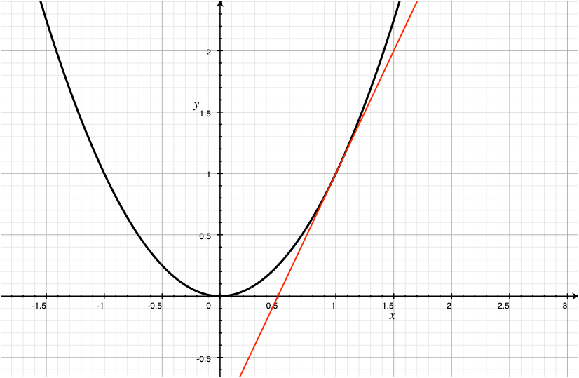
The straight line, shown in red, is a good approximation to the parabola near \(x = 1 \). The equation for the red line is \(y = 2x - 1\). Call this function \(g(x)\). It's worth taking a look at some of the values nearby.
Rather than vary x directly, it is convenient to introduce a new variable \(h\) that varies around 0, and think of \(x\) as fixed, in this example, at \(1\). The comparison of interest is between \(f(x+h)\) and g(x+h). The table below gives the results for the 21 values of \(h = -0.10, -0.09, \ldots , 0.09, 0.10 \) and compare \(f(x+h)\) with \(g(x+h) = 1 + 2h \) (Remember x=1 and substitute into the formula for g)
| h | f(x+h) | g(x+h) | f(x+h)-g(x+h) | \( \frac{f(x+h)-g(x+h)}{h} \) |
| -0.10 | 0.8100 | 0.8000 | 0.0100 | -0.1000 |
| -0.09 | 0.8281 | 0.8200 | 0.0081 | -0.0900 |
| -0.08 | 0.8464 | 0.8400 | 0.0064 | -0.0800 |
| -0.07 | 0.8649 | 0.8600 | 0.0049 | -0.0700 |
| -0.06 | 0.8836 | 0.8800 | 0.0036 | -0.0600 |
| -0.05 | 0.9025 | 0.9000 | 0.0025 | -0.0500 |
| -0.04 | 0.9216 | 0.9200 | 0.0016 | -0.0400 |
| -0.03 | 0.9409 | 0.9400 | 0.0009 | -0.0300 |
| -0.02 | 0.9604 | 0.9600 | 0.0004 | -0.0200 |
| -0.01 | 0.9801 | 0.9800 | 0.0001 | -0.0100 |
| 0.00 | 1.0000 | 1.0000 | 0.0000 | Undefined |
| 0.01 | 1.0201 | 1.0200 | 0.0001 | 0.0100 |
| 0.02 | 1.0404 | 1.0400 | 0.0004 | 0.0200 |
| 0.03 | 1.0609 | 1.0600 | 0.0009 | 0.0300 |
| 0.04 | 1.0816 | 1.0800 | 0.0016 | 0.0400 |
| 0.05 | 1.1025 | 1.1000 | 0.0025 | 0.0500 |
| 0.06 | 1.1236 | 1.1200 | 0.0036 | 0.0600 |
| 0.07 | 1.1449 | 1.1400 | 0.0049 | 0.0700 |
| 0.08 | 1.1664 | 1.1600 | 0.0064 | 0.0800 |
| 0.09 | 1.1881 | 1.1800 | 0.0081 | 0.0900 |
| 0.10 | 1.2100 | 1.2000 | 0.0100 | 0.1000 |
The fourth column, headed \(f(x+h)-g(x+h)\) shows the error in the approximation, and it is smaller when \(h\) is close to 0. By itself, this is not surprising. Cut the distance to from \(x=1\) and the approximation should get better. The surprise is in the fifth column, headed \( \frac{f(x+h)-g(x+h)}{h} \), that shows that the difference gets small even relative to \(h\).
In the example we took a function \(y=f(x)\) and showed a showed a good linear approximation to that function around a fixed value of \(x\). Fixing \(x\) and introducing the variable \(h\) to represent the variation, the approximation to \(f(x+h)\) is \(f(x) + b*h\) The derivative of \(f\) at the point \(x\) is the value \(b\).
The analytic basis for finding the derivative will be covered later. For now, using the approximations to argue for the reasonableness of the rules presented below, rules for computing the derivative of some simple functions will be developed.
Let \(f(x) = c\) for all \(x\) where \(c\) is a constant. \(f(x+h) = c = f(x)+0*h\) is a linear approximation. In fact, it is exact, and it is reasonable to take the derivative to be 0.
Rule 1: The derivative of a constant function is 0.
Let \(f(x) = x \). The \(f(x+h) = x+h = f(x) + 1*h\) which suggests that the derivative of the identity function is 1.
Rule 2: The derivative of the function \(f(x) = x\) is 1.
The derivative of \(f\) at \(x\) is denoted \(f'(x)\). There is the alternate Leibniz notation which is sometimes helpful: \(\frac{d f(x)}{dx} \), and sometimes when we want to emphasize the value of \(x\) \[ \left. \frac{df(x)}{dx} \right|_{x=7} \]
Suppose \(f'(x) = a \) and \(g'(x) = b \). Then the linear approximations are, \(f(x+h) \approx f(x)+ah\) and \(g(x+h) \approx g(x)+bh\). Apply the definition and simplify: \[(f+g)(x+h) = f(x+h) + g(x+h) \approx f(x) + ah + g(x) + bh = (f+g)(x) + (a+b)h \] And it is reasonable to take the derivative of the sum of functions to be the sum of the derivatives.
Rule 3: \((f+g)' = f' + g'\).
Suppose \(f'(x) = a \) and \(g'(x) = b \). Then the linear approximations are, \(f(x+h) \approx f(x)+ah\) and \(g(x+h) \approx g(x)+bh\). Apply the definition and simplify: \[(fg)(x+h) = f(x+h)g(x+h) \approx (f(x) + ah)(g(x) + bh) = f(x)g(x) +f(x)bh + g(x)ah + abh^2 = (fg)(x) + (f(x)b + ag(x))h + abh^2 \] If we ignore the last term \(abh^2\), then the derivative of the product can be guessed at at \((fg)' = f'g + f g'\), or using Leibniz notation \(\frac{dfg}{dx} = \frac{df}{dx} g + f \frac{dg}{dx} \).
The term \(abh^2\) can in fact be ignored, because we are interested in the approximation for small values of \(h\). If \(h\) is small, then \(h^2\) is very small. So ignoring it won't make much of a difference. This justifies the last rule of the section.
Rule 4: \((fg)' = f'g + fg'\).
The 4 rules are enough to compute the derivatives of polynomials. Induction says that is something is true for \(n=1\) and if it is true for \(n\) then it will be true for \(n+1\), then it will be true for all numbers \(n = 1, 2, 3, \ldots \).
\(x^0 = 1\) is a constant so by rule 1 HERE
If the derivative of \(f\) is defined at \(x\), and has value \(r\) then \(f(x)+ rh \approx f(x+h)\) for small values of \(h\).
In practice it becomes important to compute the formula for the derivative and sometimes to compute numerical values. Once the foundation is developed the rules for computing the formulas are proved as theorems, and these then form the basis for computing derivatives. Only rarely is it necessary to go back to the defining limits. Using the approximation formula as a guide for understanding, the rules can be specified directly and then used for calculation.
The integral of a function can be thought of as a sum. For example to compute the energy consumed by an electrical device multiply the voltage by the amperage by the time. If the voltage and amperage are constant this is not a hard calculation. The these quantities are varying the calculation gets harder. Another example is to compute the volume of a barrel. If it's a cylinder the calculation isn't too bad, but if it is barrel shaped there is more work to be done.
Computing the area under the graph of a function gets at the essense of these sorts of problem.
The constant function \( f(x) = c \) for all \(x\). Plugging into the approximatiom formula \( f(x+h) \approx f(x) + rh \) for some value of \(r\). \(f(x+h) = f(x) = c\) so \(r = 0\). This motivates the first formal rule: the derivative of a constant is 0.
The identity function \( f(x) = x \) for all \(x\) The approximation formula is \( f(x+h) = f(x) + rh \). Substituting in the definition of \(f\) gives \(x+h = x + rh\) so \(r = 1\). The second formal rule is that the derivative of the identity is 1.
Sums. If \(f'(x) = r\) and \(g'(x) = s\) then \((f+g)(x+h) = f(x+h) + g(x+h) \approx f(x)+rh + g(x) + sh = (f+g)(x) + (r+s)h\). This gives the third formal rule that the derivative of a sum is the sum of the derivatives, \((f+g)' = f' + g'\).
Products. If \(f'(x) = r\) and \(g'(x) = s\) then \((fg)(x+h) = f(x+h)g(x+h) \approx (f(x)+rh)(g(x)+sh) = f(x)g(x)+f(x)sh + g(x)rh +rsh^2\). If \(h\) is small then \(h^2\) is very small so we can neglect the term \(rsh^2\). Thus the approximation can be written \((fg)(x) + (f(x)s + rg(x))h\). Using dots for multiplication helps readability. This motivates the product rule \( (f \cdot g)' = f' \cdot g + f \cdot g' \).
Composition. \(f(g(x+h)) \approx f(g(x)+sh) \approx f(g(x))+rsh \) which suggests that \((f \circ g)'(x) = f' \circ g(x) \cdot g'(x) \). This is the fifth rule \((f \circ g)' = (f' \circ g) \cdot g' \).
Applying the product rule to \(\frac{dx^2}{dx}\) gives \( x \cdot \frac{dx}{dx} + \frac{dx}{dx} \cdot x = 2x = 2x^1\). Assuming that \( (x^j)' = j x ^{j-1} \) is true for \( j = 1, 2, \ldots , n \) applying the product rule to \((x^{n+1})' = (x \cdot x^n)' = 1 \cdot x^n + x \cdot nx^{n-1} = (n+1)x^n \). Which verifies that \((x^n)' = nx^{n-1} \) for all positive integers.
Together with the addition rule we can differentiate any polynomial.
Use the binomial formula for another justification of this rule.
Let \( f(x) = \frac{1}{x} \). \( f(x) \) can also be written as \( x^{-1} \). Using the polynomial rule gives \( f'(x) = (x^{-1})' = -1 \cdot x ^ {-2} \). One way to check this is to let \( g(x) = x \) then \((fg)(x) = 1\). Taking derivatives of both sides \[ \begin{eqnarray*} (f'g)(x) + (fg')(x) & = & 0 \\ f'(x) \cdot x + f(x) \cdot 1 & = & 0 \\ f'(x) \cdot x + \frac{1}{x} & = & 0 \\ f'(x) \cdot x & = & \frac{-1}{x} \\ f'(x) & = & \frac{-1}{x^2} \end{eqnarray*} \] Showing that the power rule holds for \(x^{-1}\).
Show that \(\frac{d}{dx} x^{n} = nx^{n-1} \) for \( n = -2, -3, \ldots \).
Let \(f(x) = \frac{1}{x} \), show
The quotient of two functions \(\frac{f}{g} = f \cdot h \circ g \) when \(h(x) = \frac{1}{x} \). The derivative can be computed \[ \begin{eqnarray*} \frac{d}{dx} \frac{f(x)}{g(x)} & = & f'(x) \cdot h(g(x)) + f(x) \cdot h'(g(x)) \cdot g'(x) \\ & = & f'(x) \cdot \frac{1}{g(x)} + f(x) \cdot frac{-1}{g^2(x)} \cdot g'(x) \\ & = & \frac{f'(x) \cdot g(x) - f(x) \cdot g'(x)}{g^2(x)} \end{eqnarray*} \]
Return to the table of contents